
August 11, 2017
Special recap of this past winter
Below I try to weave a narrative of this past winter. The predominant thinking in the field is that sequential weather or synoptic events are random and unrelated known as chaos theory. However I have tried to show how different events throughout the winter are related and one follows the next more akin to a domino effect and events at the beginning of the winter are responsible for events at the end of the winter. I feel that this is a unique perspective on the winter season that can only be accomplished through consideration of troposphere-stratosphere coupling and involvement of the polar vortex. Both the hemispheric weather and the polar vortex showed extreme variability this winter and an in-depth understanding of the variability of each is impossible without the other. Such an explanation of the extreme variability is much more difficult using El Nino Southern Oscillation (ENSO), which showed very little variability throughout the winter.
Summary
- Winter 2016/17 was characterized by warmth in Central and Eastern North America, Northern Europe, Central and East Asia but cold in much of Europe, the Middle East and Siberia.
- The dominant story in the fall was extensive October Siberian snow cover that resulted in very cold temperatures across Northern Asia in November.
- The strong temperature gradient across Asia provided fuel for a strong North Pacific Jet Stream that cooled sea surface temperatures in the mid-latitudes of the North Pacific.
- The strong sea surface temperature (SST) gradient in the mid-latitudes of the North Pacific maintained an active Jet Stream into the West Coast of the United States (US) resulting in cool temperatures and record rainfall along the US West Coast but flooded the rest of North America east of the Rockies with mild, maritime air.
- Low sea ice in the Barents Kara seas helped anchor high pressure in the region, especially Northern Europe, for much of the winter. Northeasterly flow around the high pressure, especially in January, resulted in an overall cold winter for Europe except near the center of the high across Northern Europe.
- Analysis of the relationship between warming in the Barents-Kara Seas and surface temperatures across the Northern Hemisphere (NH) suggest the record low sea ice in the Barents-Kara seas may have contributed to warm temperatures both across Northern Europe and the Eastern US.
- Extensive Eurasian snow cover and low Arctic sea ice in October contributed to an early and strong Siberian high that favors a weak polar vortex. However the most impressive polar vortex weakening and subsequent coupling with the troposphere took place in the fall followed by a relatively strong polar vortex and a positive Arctic Oscillation (AO) in mid-winter. This contributed to front ending cold temperatures with the back end relatively mild across the NH.
- There was a brief major mid winter warming (wind reversal at 60°N and 10 hPa) in early February but its impact was relatively minor and short lived in the troposphere. It is possible that the westerly phase of the quasi-biennial oscillation played a role in reducing the strength and duration of the major warming and its impact on the weather.
- Despite the La Niña, California received record rainfall and snowfall, which spilled over to many western states. Few could have anticipated prior to the winter that the severe drought (at least as defined by the US Drought Monitor) in California would be erased in a single season.
Boundary Forcings
The climate community focuses on El Niño/Southern Oscillation or ENSO in making seasonal forecasts and a La Niña event was predicted by the models for winter 2016/17. La Niña favors colder temperatures in the Northwestern US and warmer temperatures in the Southeastern US. La Niña also favors heavy precipitation in the Northwestern US and lighter precipitation in the Southwestern US including California. During the winter of 2016/17 weak La Niña conditions were observed.
Though at AER we use ENSO in producing seasonal forecasts, we have pioneered the use of Arctic boundary forcings in winter seasonal forecasting including Arctic sea ice but especially Eurasian snow cover in October. We have demonstrated using observational analysis and model perturbation experiments that extensive Eurasian October snow cover is related to/can force a strengthened Siberian high, increased poleward heat flux, a weak PV, which culminates in an extended period of a negative AO. A negative AO is associated with below normal temperatures in the Eastern US and Northern Eurasia including Northern Europe and East Asia. Scientists including those at AER, have shown a similar atmospheric response to low Arctic sea ice. There are different ideas how variability in Arctic sea ice might influence winter hemispheric weather but the trend has been a convergence to a similar set of mechanisms first proposed for Eurasian snow cover. Also there is growing consensus that it is Barents-Kara sea ice in the late fall and early winter that has the greatest impact across Eurasia. Therefore low Barents-Kara sea ice in November for example, favors a strengthened Siberian high, increased poleward heat flux, a weak PV and finally a negative AO. Though I am less certain that the atmospheric response from low Barents-Kara sea ice really projects onto the AO (see concluding remarks). An important point in regards to the Siberian high, it strengthens or expands northwest of the climatological center. For low snow cover and/or high sea ice the opposite occurs.
October 2016 Eurasian snow cover extent (SCE) was the third highest observed going back to 1972 (Figure 1a). Well above normal SCE favored a sudden stratospheric warming (SSW) and a weak PV in mid winter followed by a negative AO and cold temperatures across the NH mid-latitudes. September 2016 Arctic sea ice was tied for third lowest observed and November 2016 Barents-Kara sea ice was third lowest (based on my own calculations) going back to 1979 (Figure 1b). Therefore Arctic sea ice similarly favored a weak PV in mid winter followed by a negative AO and cold temperatures across the NH mid-latitudes. However during the winter Barents-Kara sea ice was the lowest ever observed from satellites by a wide margin.
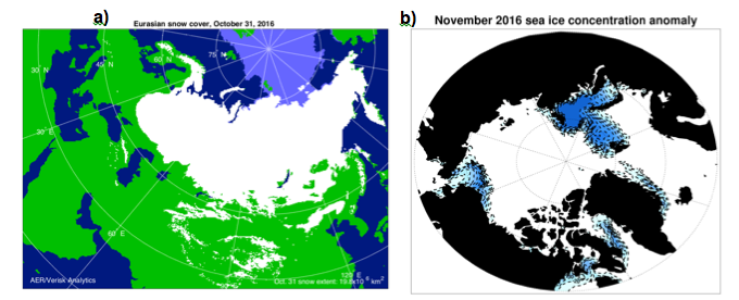
Figure 1. a) Snow cover extent across Eurasia on October 31, 2016 shown in white, Arctic sea ice shown in light blue. b) Observed Arctic sea ice extent anomalies November 2016. Negative anomalies shown in blue shading.
The quasi-biennial oscillation (QBO) was in its westerly phase. The QBO is a periodic oscillation of the zonal winds in the equatorial stratosphere and in the westerly phase the zonal winds are stronger. The westerly phase is thought to inhibit the strongest SSWs where the zonal wind reverses in direction and is referred to as a major midwinter warming.
And of course the near record warm global atmosphere and ocean provided an overall warm backdrop heading into the winter of 2016/17.
Late fall/early Winter
As mentioned above, October 2016 Eurasian snow cover was the third highest observed going back to 1972. Above normal snow cover across Siberia in October favors a strengthened Siberian high in November and into December with the largest positive sea level pressure anomalies northwest of the climatological center (see Figure 2a taken from Cohen et al. 2014). But with the quick start to the Siberian snow cover advance, a strong Siberian high did not wait until November to appear but rather became well established relatively early in October 2016 (Figure 2b). This formed a strong tripole pattern, which is optimal for forcing increased vertical transfer of Rossby wave energy (vertical wave activity flux or WAFz) and poleward heat flux even though it was about a month early relative to climatology.
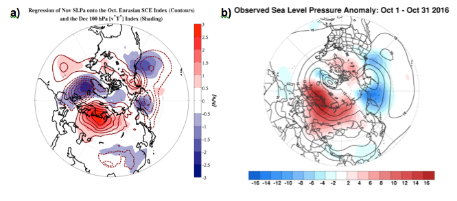
Figure 2. a) Regression of November SLP anomalies (hPa) onto October monthly mean, October Eurasian SCE (contouring) and December meridional heat flux anomalies at 100 hPa, averaged between 40-80°N (shading). b) Observed average sea level pressure (hPa; contours) and sea level ressure anomalies (hPa; shading) across the Northern Hemisphere from October 1, 2016 through October 31, 2016.
The WAFz plot in Figure 3 shows the active WAFZ in late October, which was record strong for the date. Strong upward WAFz absorbed in the stratosphere weakened the polar vortex and the plot of the polar cap geopotential height anomalies (PCH) in Figure 4 shows that the stratospheric polar vortex became exceptionally weak at the end of October and even resulted in an unprecedented polar vortex split at the end of October and the beginning of November. Figure 5a shows the 10 hPa geopotential height in early November and a split PV is clearly visible with one PV center over the Urals and the other PV center over Hudson Bay. The weak PV that peaked at the end of October lasted the entire month of November and propagated to the surface in early November, late November and early December (Figure 4).
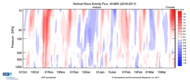
Figure 3. Observed daily vertical component of the wave activity flux (WAFz) standardized anomalies, averaged poleward of 40-80°N from October 1 through March 31 (data for first week is missing).
The weak PV, the downward propagation of positive PCHs from the stratosphere to the troposphere and a negative AO resulted in widespread and unseasonably cold air across the Eurasian continent, especially in Western Siberia in November (Figure 6a).
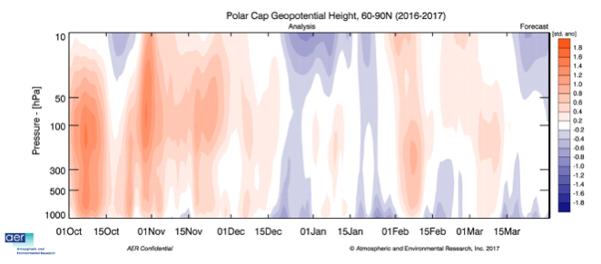
Figure 4. Observed daily polar cap height (i.e, area-averaged geopotential heights poleward of 60°N) standardized anomalies from October 1 through March 31 (data for first week is missing).
In my opinion the rapid advance of snow cover, the strengthened and westward displaced Siberian high, the active upward WAF, the weak PV, the negative AO and cold temperatures especially in Siberia was a textbook example of snow-atmosphere coupling with one exception – the timing. Typically the weak PV peaks in mid to late January but last fall and winter the weak PV peaked in late October, three months early. Typically the AO averages negative for four to six weeks following a weak PV accompanied by colder than normal temperatures. This was observed from late October through mid-December in 2016 matching the expectations but two to three months early. The cold was focused across Eurasia, which is typical for weak polar vortex events.
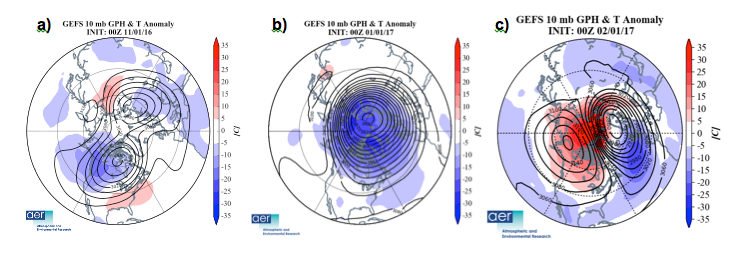
Figure 5. a) Analyzed 10 hPa geopotential heights (dam; contours) and geopotential height anomalies (m; shading) across the Northern Hemisphere for 1 November 2016 b) same as a) except analyzed for 1 January 2017 c) same as a) except analyzed for 1 February 2017.
The cold did eventually make its way to North America with the last downward propagation of the circulation anomalies associated with the weak PV in early December (Figure 6b). But in my opinion the greatest impact on North American winter weather from the rapid advance of Siberian snow cover was not through the stratosphere but through the troposphere. With the recovery of the PV and the conclusion of the last downward propagation the impact through the stratospheric PV on NH winter weather was finished by mid-December.
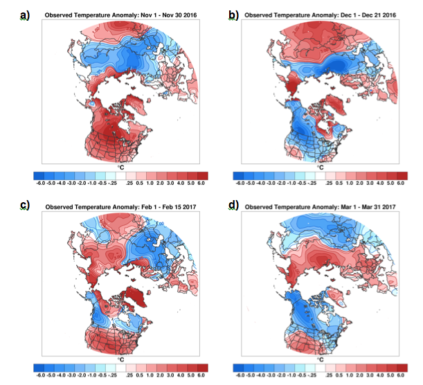
Figure 6. a) Observed surface temperature anomalies ((°C; shading) for November 1-31, 2016 b) observed surface temperature anomalies ((°C; shading) for December 1-21, 2016 c) observed surface temperature anomalies ((°C; shading) for February 1-15, 2017 c) observed surface temperature anomalies ((°C; shading) for March 1-31, 2017.
But in my opinion there was a clear and much more lasting impact on North American weather excited by the rapid advance in Siberian snow cover involving North Pacific SSTs and the North Pacific Jet Stream. The rapid advance of snow cover across Siberia in October resulted in well below normal temperatures across Siberia in November (Figure 6a). Meanwhile temperatures remained well above normal further south across China. This amplified the meridional temperature gradient across East Asia, supercharging the East Asian Jet. This jet then extended east out over the North Pacific in November (Figure 7a).
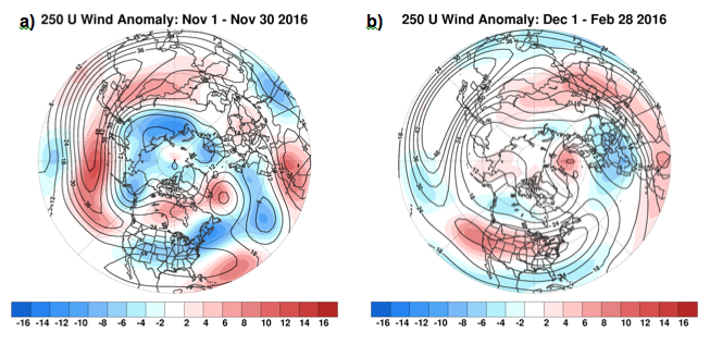
Figure 7. a) Observed 250 hPa zonal wind (ms-2; contours) and 250 hPa zonal wind anomalies (ms-2; shading) across the Northern Hemisphere from November 1-30, 2016 through February 28, 2016. b) Same as a)except for December 1, 2016 through February 28, 2017.
The strengthened westerly wind over the North Pacific reversed the warmest SST anomalies in the NH mid-latitudes to the coldest SST anomalies in the NH mid-latitudes in just one month from October to November (Figure 8). This pattern of cold SSTs to the north (ceentered around 45°N) and warmer SSTs to the south (centered around 30°N) strengthened the North Pacific jet (centered around 35°N) throughout the winter. The dipole of cold SSTs to the north and warm SSTs to the south drifted east throughout the winter and with it the core of the jet drifted east and the strongest jet stream anomalies during the winter were along the west coast of North America centered over California (Figure 7b). The anomalously strong jet not only resulted in record rainfall and snowfall for California despite the La Niña but flooded North America with mild, maritime air east of the Rockies leading to an overall mild winter for the Eastern US and Eastern Canada.
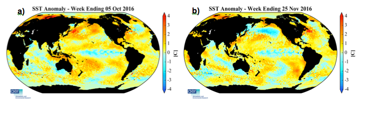
Figure 8. a) The weekly-mean global SST anomalies ending 5 October 2016. b) The weekly-mean global SST anomalies ending 25 November 2016. Data from NOAA OI High-Resolution dataset.
Mid winter
With the atmospheric response to the rapid snow cover advance across Siberia in October including the strong transfer of energy from the troposphere to the stratosphere, the weak PV and the negative AO concluded by the middle of December the opposite occurred with a positive AO, decreased energy transfer from the troposphere to the stratosphere, a strengthened PV and concluding with a positive AO starting in mid-December through the end of January (Figures 3, 4).
In the PCH plot a troposphere-stratosphere-troposphere coupling event is clearly seen in the PCH plot (Figure 4) starting with cold tropospheric PCH in late December. An overall positive AO can be seen in the 500 hPa geopotential height in late December (Figure 9a). The high latitudes are dominated by low geopotential heights with one exception - positive heights in the Barents-Kara-Laptev Seas and Northern Europe. I would argue that the low sea ice in the Barents-Kara seas contributed to the ridging/high pressure in the region. The NH atmospheric circulation is not conducive to energy transfer from the troposphere to the stratosphere and negative WAFz anomalies were observed the end of December (Figure 3). This allowed the stratospheric PV to spin up and the PV remained strong from late December through late January (Figure 5b).
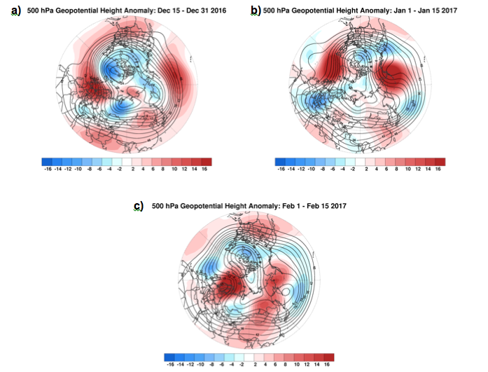
Figure 9. a) Observed average 500 hPa geopotential heights (dam; contours) and geopotential height anomalies (m; shading) across the Northern Hemisphere from December 15-31 2016 b) same as a) except for January 1-15, 2017 and c) same as a) except for February 1-15, 2017.
A cold/strong PV in both the troposphere and stratosphere at the end of December allowed for an overall mild pattern across much of the NH in late December. However often when the stratospheric PV is transitioning from weak to strong or strong to weak the tropospheric PV transitions in the opposite direction. From the end of December through mid-January while the stratospheric PCHs turned cold, the tropospheric PCHs warmed (though only modestly). It did allow for an increase in positive heights across the high latitudes though only regionally. Positive geopotential height anomalies over the Barents-Kara seas and south of Greenland to Iceland (Figure 9b) forces northerly flow over Europe resulting in cold temperatures over much of Europe (Figure 6b). This cold air outbreak across Europe is strong enough to dominate the winter means providing Europe with an overall cold winter. The cold was accompanied by heavy snowfalls even to regions not accustomed to snow such as the Greek Islands, Southern Spain and even the Sahara Desert. An exception is Northern Europe where positive heights and/or westerly flow results in warm temperatures. Another region of high heights/ridging is near Alaska (Figure 9b) forcing northerly flow over the West Coast of North America resulting in cold temperatures over Southwestern Canada and the Northwestern US (Figure 6b). Further east, ridging and southwesterly flow (Figure 9b) result in mild temperatures for the Eastern US and Eastern Canada (Figure 6b).
Late winter
By the end of the January the cold/strong PCHs in stratosphere descend from the stratosphere to the troposphere (Figure 4) completing the second troposphere-stratosphere-troposphere coupling event of the winter, which began in late December. Once again the high latitudes of the troposphere are dominated by low heights and a positive AO and an overall mild pattern across the NH mid-latitudes. However positive height anomalies do coalesce across Northern Europe (Figure 9c). Though not ideal, the atmospheric circulation projects strongly enough onto the tropospheric precursor pattern (Figure 2a) to force more upward WAF from the troposphere to the stratosphere in late January (Figure 3). The WAFz is strong enough to force a minimal major midwinter warming in early February as the stratospheric PV is displaced off the North Pole and near Northern Scandinavia (Figure 5c).
The warm PCHs and negative AO quickly descended from the stratosphere to the troposphere in early February (Figure 4). This once again allowed positive geopotential height anomalies to encroach on the high latitudes with the strongest positive anomalies in the NH centered across Northern Europe and the Barents-Kara seas. I would argue that the consistent ridging/positive geopotential height anomalies in the Barents-Kara Seas, the North Atlantic and Northern Europe was related to low sea ice in the Barents-Kara Seas and warm SSTs in the northern North Atlantic. The ridging in the northern North Atlantic pushed far enough north, to force troughing in Eastern Canada and the Northeastern US in early February. The northerly flow brought the return of cold air to Eastern Canada and more seasonable temperatures to the Northeastern US (Figure 6c). Though the cold air in the Northeastern US was modest, the pattern did result in heavy snowfalls and even record snow depths to parts of Maine and New Hampshire.
However the warm PCHs/negative AO did not last very long and by mid to late February cold PCHs/positive AO had returned along with another mild pattern across the NH continents. I do not have a good explanation for the short duration of the warm tropospheric PCHs and the negative AO following the stratospheric warming/weak stratospheric PV in early February. It is likely related to lack of high pressure over the central Arctic that instead remained at the periphery either in the northern North Atlantic and/or the northern North Pacific. The SSTs near Svalbard, Iceland and Alaska were the warmest across the NH and it could be that they helped anchor ridging/positive geopotential height anomalies near those locations that never could coalesce around the North Pole or closer to Greenland as is typical during a negative AO, despite repeated stratospheric warmings. It is possible that the westerly QBO played a role by limiting the WAFz absorbed in the polar stratosphere and limiting the amplitude and duration of any stratospheric warmings.
With ridging/positive geopotential height anomalies centered near Northern Europe and the Barents-Kara seas the first half of February (Figure 9c) the atmospheric circulation projected onto the tropospheric precursor pattern (Figure 2a) favoring more active WAFz yet again. Increased upward WAFz the second half of February favors cold tropospheric PCHs, a positive AO and an overall mild pattern across the NH continents. However it also favors the opposite in the stratosphere with warming PCHs and a negative stratospheric AO, which peaked at the end of February. Downward propagation of the warm PCHs and negative AO from the stratosphere to the troposphere quickly ensued in early March. This concluded at least three troposphere-stratosphere-troposphere coupling events throughout the fall-winter season. The first was a warm PCH/weak PV event from late October through early December, the second was a cold PCH/strong PV event from late December the end of January and the third was a warm PCH/weak PV event from early February through early March. There is even a likely fourth event consisting of a warm PCH/weak PV event mid January through mid February, though it is not as clear from the PCH plot as the other three.
The warm PCHs and the negative AO in early March allowed for cold air to return to the NH continents. One important difference with this event from the previous winter negative AO events, above normal geopotential heights were not centered near Northern Europe but over Greenland instead. This allowed for cold air to become more widespread across eastern North America and the month of March was cold for most of Canada and the Eastern US (Figure 6d). It also resulted in another record breaking snowstorm for the Northeastern US. With Binghamton, New York recording its greatest snowfall ever capping a ecord breaking snowfall season. High pressure across Siberia also advected cold air further south across much of southern Asia (Figure 6d).
Observed winter circulation
It is my opinion that high latitude boundary forcings play a key role in the atmospheric winter circulation of the mid-latitudes. I explained the dynamic twist and turns of the PV, the AO, high latitude blocking and large-scale temperature anomalies using boundary forcings of the high latitudes. For the winter of 2016/17, I argued that low Barents-Kara sea ice coupled with warm SSTs in the northern North Atlantic, and warm SSTs in the northern North Pacific were most important for anchoring ridging/positive geopotential height anomalies near Northern Europe and near Alaska respectively (Figure 10). Northerly flow and low heights downstream of the ridge center over Northern Europe provided below normal winter temperatures to Europe, Western Asia and the Middle East. The second ridge center near the Aleutians, provided below normal winter temperatures to the west coast of North America including Alaska. The last region that recorded below normal winter temperatures was Siberia. I would attribute the cold temperatures in Siberia to the trough in Western Russia and the rapid advance of snow cover across the region in the fall season. Winter temperatures in Siberia are highly correlated with snow cover extent across Siberia in the fall and the coldest winter temperatures across Siberia were front-loaded (Figure 6).
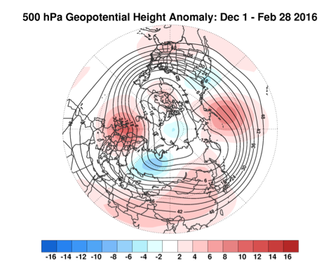
Figure 10. a) Observed average 500 hPa geopotential heights (dam; contours) and geopotential height anomalies (m; shading) across the Northern Hemisphere from December 1, 2016 through February 28, 2017.
The other high latitude boundary forcing that I consider important for the NH winter weather is Siberian snow cover. This past October one of the most rapid advances in snow cover extent ever was observed. This resulted in extreme and widespread cold temperatures in the month of November across Siberia. The strong meridional temperature gradient energized the East Asia Jet that extended into the North Pacific. Strong westerly flow across the mid-latitudes of the North Pacific rapidly cooled SSTs first in the western North Pacific and then in the eastern North Pacific. The resultant jet streak propagated eastward with the SST gradient. Over the entire winter the strongest westerly wind anomalies were along the California Coast bringing record rainfall and snowfall to the state. In addition, the strong jet acted as a hose of mild, maritime air, flooding North America east of the Rockies with repeated periods of well above normal temperatures. This tropospheric pathway has been shown in modeling experiments by Gina Henderson et al. 2013 (http://journals.ametsoc.org/doi/abs/10.1175/JCLI-D-11-00465.1).
The boundary forcing in the tropics considered dominant in forcing seasonal climate is ENSO and dynamical model forecasts were driven predominately by a predicted La Niña during the winter. Surface temperature anomalies with below normal temperatures in the Pacific Northwest and Western Canada with above normal temperatures in the Southeastern US and even extending further north into the Northeastern US and Eastern Canada is consistent with North American temperature variability associated with La Niña. However the precipitation anomalies observed across the Western US is almost 100% out of phase with precipitation variability associated with La Niña (Figure 11). The precipitation forecast was for dry in California with wet further north into the Pacific Northwest and British Columbia when in actuality it was record wet in California and dry further north in Washington State and British Columbia. Also the Jet Stream anomalies in the North Pacific in winter 2016/17 were not consistent with canonical Jet Stream anomalies in the North Pacific associated with La Niña. During La Niña, the Jet Stream strengthens on the poleward side, As shown earlier (Figure 7) there was no strengthening of the Jet Stream in the North Pacific on the poleward (or equatorward side) but rather it extended further east into California.
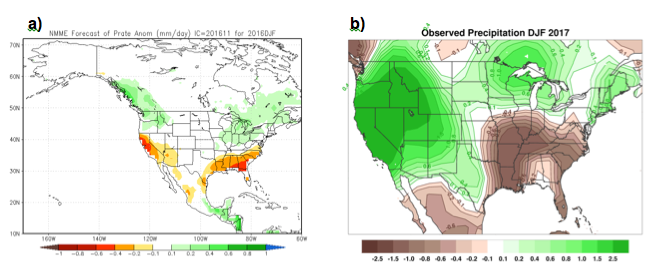
Figure 11. a) NMME predicted precipitation rate for North America from December 1, 2016 through February 28, 2017 b) observed average precipitation anomalies (inches; contours) across the United States from December 1, 2016 through February 28, 2017.
The “rinse, repeat” of tropospheric-stratosphere coupling of winter 2016/17 described in detail above, occurring three to four times, reminds me of winter 2015/16. Why accelerated troposphere-stratosphere coupling has occurred the past two winters, in my opinion is an important question and I don’t have a good answer. Though both winters were characterized by low Barents-Kara sea ice, strong blocking near the Urals/Barents-Kara seas that is so favorable for WAFz/poleward heat transport. This may have prohibited high pressure from organizing over the North Pole, which would have resulted in a quieter period of WAFz and fewer tropospheric-stratosphere-troposphere coupling events the past two winters.
Winter forecasts
Before the winter I published the AER winter forecast on the National Science Foundation website, which is still there and here I have included the NH version of the forecast (Figure 12a). The main predictors in the AER forecast were October Eurasian snow cover, Arctic sea ice and La Niña. Snow cover was high and sea ice low so therefore the model forecast were consistent with a weak polar vortex and a negative AO. The model predicted cold temperatures across Northern Asia, Europe and most of the eastern one third of the US, and the forecast of La Niña contributed to cold temperatures in the Northwestern US and Western Canada as well. Much of the remainder of the NH was predicted to be mild. The observed winter temperatures are also shown in Figure 12b. The model forecast was mixed with the model performing best across Siberia, parts of Europe and western North America. The biggest model error was that temperatures were generally too cold compared to the observations. In Eurasia the model missed the warm temperatures across Northern Europe. In North America the largest error were the observed warm temperatures throughout the Eastern US.
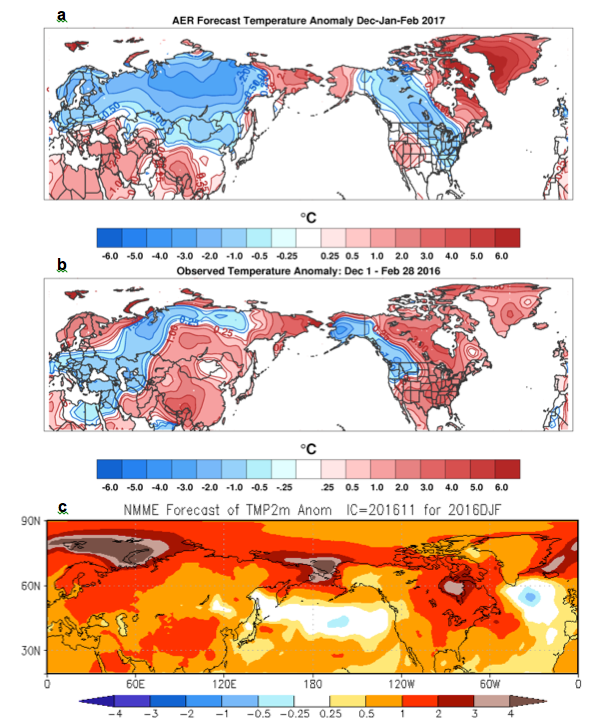
Both the extensive Eurasian snow cover and low Arctic sea ice favor a strengthened Siberian high. But typically the center of the high is over the Arctic Ocean, which results in northerly flow across East Asia and easterly flow across Europe and cold temperatures stretching across much of northern Eurasia. However this winter the center of the high was shifted west over Northern Europe. This still created northerly flow and therefore cold temperatures across Central and Eastern Europe, western Asia and even Siberia. However Northern Europe in the center of the ridging, experienced an overall mild winter. Also given that the ridging was so far west the trough more typically centered in East Asia was centered in West Asia with more ridging and warm temperatures across East Asia (Figure 10).
Figure 12. a) AER Forecasted surface temperature anomalies ((°C; shading) for December 1, 2016 through February 28, 2017 b) observed surface temperature anomalies ((°C; shading) for December 1, 2016 through February 28, 2017 c) NMME Forecasted surface temperature anomalies (°C; shading) for December 1, 2016 through February 28, 2017.
The too cold temperatures predicted in the Eastern US were a combination of the ridging near Alaska being too far southwest to drive consistent cold air into the eastern US and the strong jet streak over California hosing North America east of the Rockies with mild, maritime air.
The national multi-model ensemble (NMME) forecast for NH temperatures is included in Figure 12c. As is the case every winter now, the dynamical models predict universal above normal temperatures across the NH continents. And once again the NMME winter temperature forecasts are in general too warm. I attribute this consistent model error to model deficiencies in simulating high latitude surface-atmosphere coupling. If feel like I am in the minority with this opinion but how else to explain the very consistent model error.
Concluding remarks
Leading into winter 2016/17 I was more confident in the AER winter forecast than I had been leading into winter 2015/16. I thought the signal from Siberian snow cover extent in October 2016 was more robust than the signal from October 2015 and there wasn’t a strong El Niño predicted for winter 2016/17 as had been for winter 2015/16.
I do believe that there was an immediate and robust response to the rapid snow cover advance during the fall. It was atypically early, which did give me concern but I expected a scenario similar to winter 20009/10 with an early sudden stratospheric warming in the fall followed by a major mid winter warming in the winter. This did occur but the tropospheric response to both stratospheric warmings in fall and winter 2016/17 were much less robust than in winter 2009/10. One possible difference was that in winter 2009/10 the QBO was in the easterly phase and in winter 2016/17 the QBO was in the westerly phase.
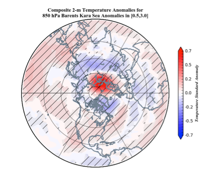
Figure 13. Composite difference in temperatures between warm and cold temperatures in the Barents-Kara seas. Plot shows association between surface temperature anomalies across the NH and in the Barents-Kara seas. Climatological averages computed over the period 1981-2010. Where difference was found to be statistically significant above 95% is hatched in light gray.
One other difference was the amplitude of the sea ice anomaly in the Barents Kara seas. Negative sea ice extent anomalies in the Barents-Kara seas region were greater in winter 2016/17 than 2009/10. In fact sea ice extent in the Barents-Kara seas was record low in winter 2016/17 by a wide margin by my own calculations. And though low sea ice extent is considered to favor cold temperatures across Asia in winter, I am starting to believe that it may favor warm temperatures in the Eastern US. In Figure 13, I show NH surface temperatures associated with warm temperatures in the Barents Kara Seas (taken from a manuscript in review). What is immediately apparent is that the hemispheric temperature pattern does not resemble the negative phase of the AO. Though it shows cold temperatures across Asia and Southern Europe it shows warm temperatures in the Eastern US and Northern Europe, similar to what was observed last winter. Of course this relationship is overly simplistic and a relationship that is apparent in one winter disappears in a different winter. Still I believe that we are just starting to comprehend the relationship between regional sea ice anomalies and winter temperatures across the NH. Improved understanding of sea ice (or lack thereof) and atmosphere coupling, I believe, provides an opportunity for improved winter predictions.